> ## Documentation Index
> Fetch the complete documentation index at: https://docs.cognite.com/llms.txt
> Use this file to discover all available pages before exploring further.
# Plot time series with legacy features
> Create dashboards and select the time series you want to plot using the time series API and custom queries.
Use this guide when you work with existing dashboards that use the legacy data model features. For time series in data model views, see [Plot time series from data model views](/cdf/dashboards/guides/grafana/timeseries).
## Create a dashboard
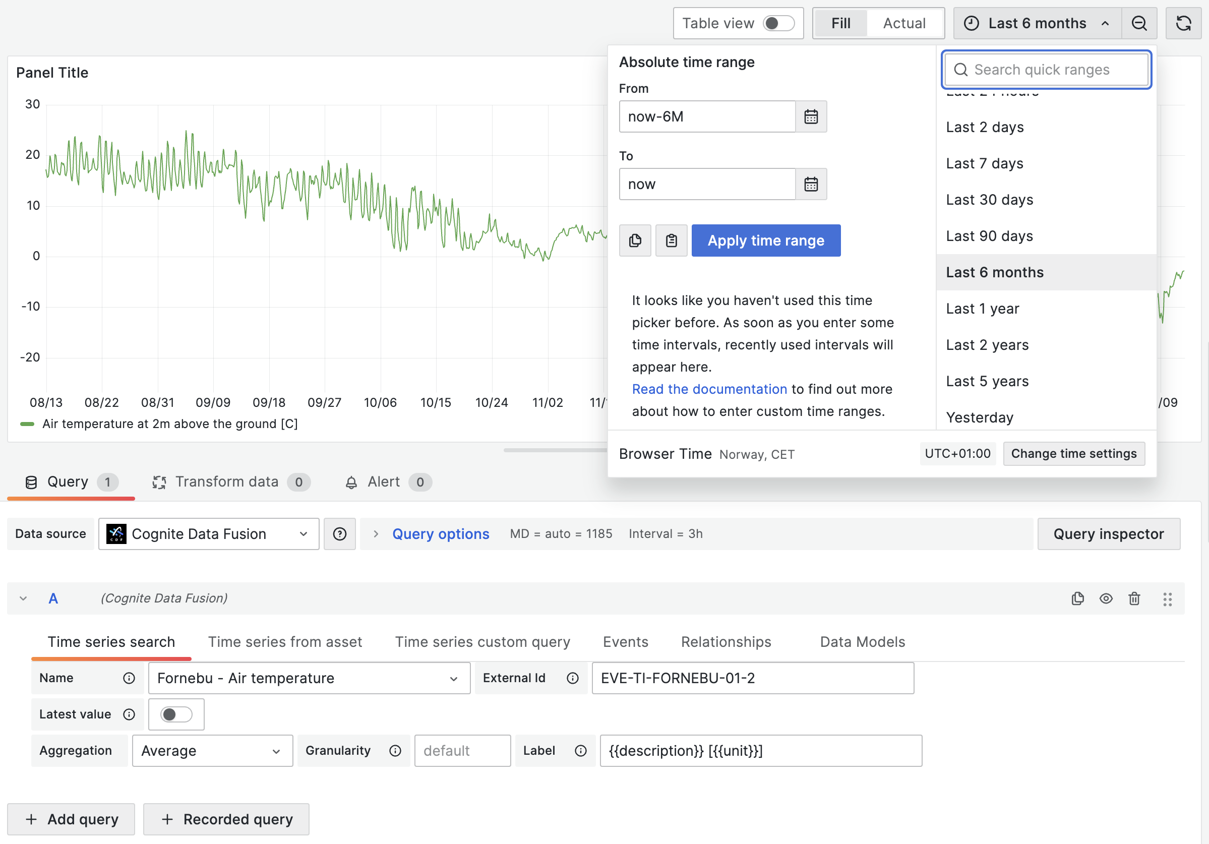
To create a dashboard with time series data from Cognite Data Fusion (CDF):
Sign in to your Grafana instance and create a dashboard.
Use the legacy query tabs below the main chart area to select time series for your dashboard:
* **Time series search** - fetch data from a specific time series. Start typing the name or description of the time series and select it from the dropdown list.
Specify [aggregation](/dev/concepts/aggregation) and [granularity](/dev/concepts/aggregation#granularity) directly in the query. By default, the aggregation is set to *average*, and the granularity is determined by the chart's selected time interval.
Optionally, set a custom **label** and use the format `{{property}}` to pull data from the time series. You can use all the available [time series properties](https://api-docs.cognite.com/20230101/tag/Time-series/operation/getTimeSeries/) to define a label, for example, `{{name}} - {{description}}` or `{{metadata.key1}}`.
* **Time series from asset** - fetch data from time series related to a specific asset. Start typing the name or description of the asset and select it from the dropdown list. Optionally, decide whether you want to include time series from sub-assets.
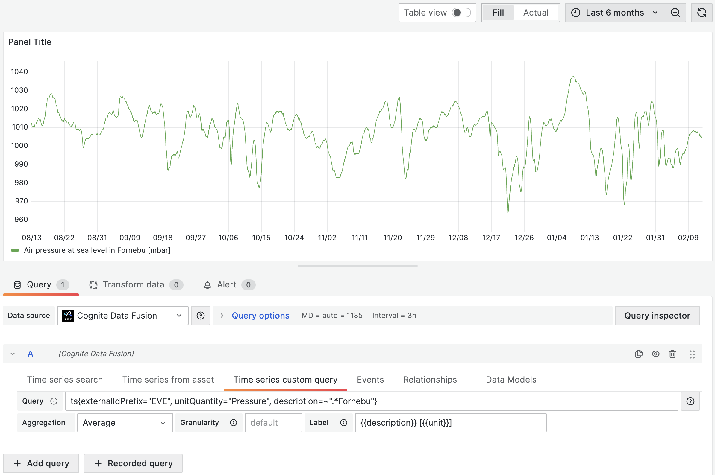
* **Time series custom query** - fetch time series that match a query. See [Use custom queries](#use-custom-queries) below.
The time series matching your selection will be rendered in the chart area. Adjust the timeframe as necessary to display relevant data.
 ## Use custom queries
Custom queries offer fine-grained control over the selection of time series data. You can use arithmetic operations, functions, and a special syntax for fetching synthetic time series. This section also outlines the limitations related to data filtering and how to effectively use regex and server-side filters.
### Define a query
To request time series, specify a query with the parameters inside. For example, to query for a time series where the `id` equals `123`, specify `ts{id=123}`.
You can request time series using `id`, `externalId`, or [time series filters](https://api-docs.cognite.com/20230101/tag/Time-series/operation/listTimeSeries/).
## Use custom queries
Custom queries offer fine-grained control over the selection of time series data. You can use arithmetic operations, functions, and a special syntax for fetching synthetic time series. This section also outlines the limitations related to data filtering and how to effectively use regex and server-side filters.
### Define a query
To request time series, specify a query with the parameters inside. For example, to query for a time series where the `id` equals `123`, specify `ts{id=123}`.
You can request time series using `id`, `externalId`, or [time series filters](https://api-docs.cognite.com/20230101/tag/Time-series/operation/listTimeSeries/).
 For **synthetic time series**, you can specify several property types:
* `bool`: `ts{isString=true}` or `ts{isStep=false}`
* `string` or `number`: `ts{id=123}` or `ts{externalId='external_123'}`
* `array`: `ts{assetIds=[123, 456]}`
* `object`: `ts{metadata={key1="value1", key2="value2"}}`
To create complex synthetic time series, you can combine the types in a single query:
```text theme={"languages":{"custom":["/_languages/kuiper.json","../_languages/kuiper.json"]}}
ts{name="test", assetSubtreeIds=[{id=123}, {externalId="external_123"}]}
```
### Filtering
Queries also support filtering based on time series properties which apply as logical `AND`. For instance, the query below finds time series:
* that belong to an asset with an `id` that equals `123`
* where `name` starts with `"Begin"`
* where `name` doesn't end with `"end"`
* where `name` doesn't equal `"Begin query"`
```text theme={"languages":{"custom":["/_languages/kuiper.json","../_languages/kuiper.json"]}}
ts{assetIds=[123], name=~"Begin.*", name!~".*end", name!="Begin query"}
```
The query syntax contains different types of equality operators:
* `=` - strict equality. Specifies parameters for the time series request to CDF. Use with filtering attributes.
* `!=` - strict inequality. Filters fetched time series by properties that aren't equal to the string. Supports string, numeric, and boolean values.
* `=~` – regex equality. Filters the fetched time series by properties that match the regular expression. Supports string values.
* `!~` - regex inequality. Filters the fetched time series by properties that don't match the regular expression. Supports string values.
You can also filter on metadata:
```text theme={"languages":{"custom":["/_languages/kuiper.json","../_languages/kuiper.json"]}}
ts{externalIdPrefix="test", metadata={key1="value1", key2=~"value2.*"}}
```
The query above requests for time series where:
* `externalIdPrefix` equals `"test"`
* `metadata.key1` equals `"value1"`
* `metadata.key2` starts with `"value2"`
### Query limitations
When performing custom queries, it's important to understand the underlying limitations for fetching time series:
* **Client-side Filtering**: The connector applies regex queries (`=~` for matches and `!~` for exclusions) and inexact inequality filters (`!=`) on the *client-side*. This process occurs after the initial retrieval of up to 1000 time series items from Cognite Data Fusion (CDF). Due to this approach, there's a possibility that not all relevant time series will be included in the fetched subset if the total number exceeds 1000.
* **Server-side Filtering**: To mitigate this limitation, it's recommended to use *server-side* filtering whenever possible. This can be achieved by applying strict equality filters (`=`) on specific [time series filter properties](https://api-docs.cognite.com/20230101/tag/Time-series/operation/listTimeSeries/). By doing so, you effectively narrow down the set of time series retrieved from CDF, ensuring that the subsequent client-side filters are applied to a more targeted dataset. This is particularly useful for ensuring that all relevant time series, especially those of interest, are included within the initial dataset fetched from CDF.
Combine *server-side* filtering with specific attributes or metadata to refine your query's scope before applying *regex* or other *client-side* filters. This approach significantly increases the chances of selecting all time series of interest in your Grafana dashboard.
### Aggregation, granularity, and alignment
You can specify aggregation and granularity for each time series using the dropdowns in the user interface.
If, for example, the aggregation is set to `average` and the granularity equals `1h`, **all** queries request datapoints with the selected aggregation and granularity. By default, aggregation with synthetic time series is aligned to Thursday 00:00:00 UTC, 1 January 1970.
With the synthetic time series query syntax, you can define aggregation, granularity, and alignment for **each time series separately**:
```text theme={"languages":{"custom":["/_languages/kuiper.json","../_languages/kuiper.json"]}}
ts{externalId='houston.ro.REMOTE_AI[34]', alignment=1599609600000, aggregate='average', granularity='24h'}
```
The query above overrides the aggregation and granularity values set in the user interface. See the API documentation for a list of [supported aggregates](/api-reference/concepts/20230101/synthetic-time-series#aggregation).
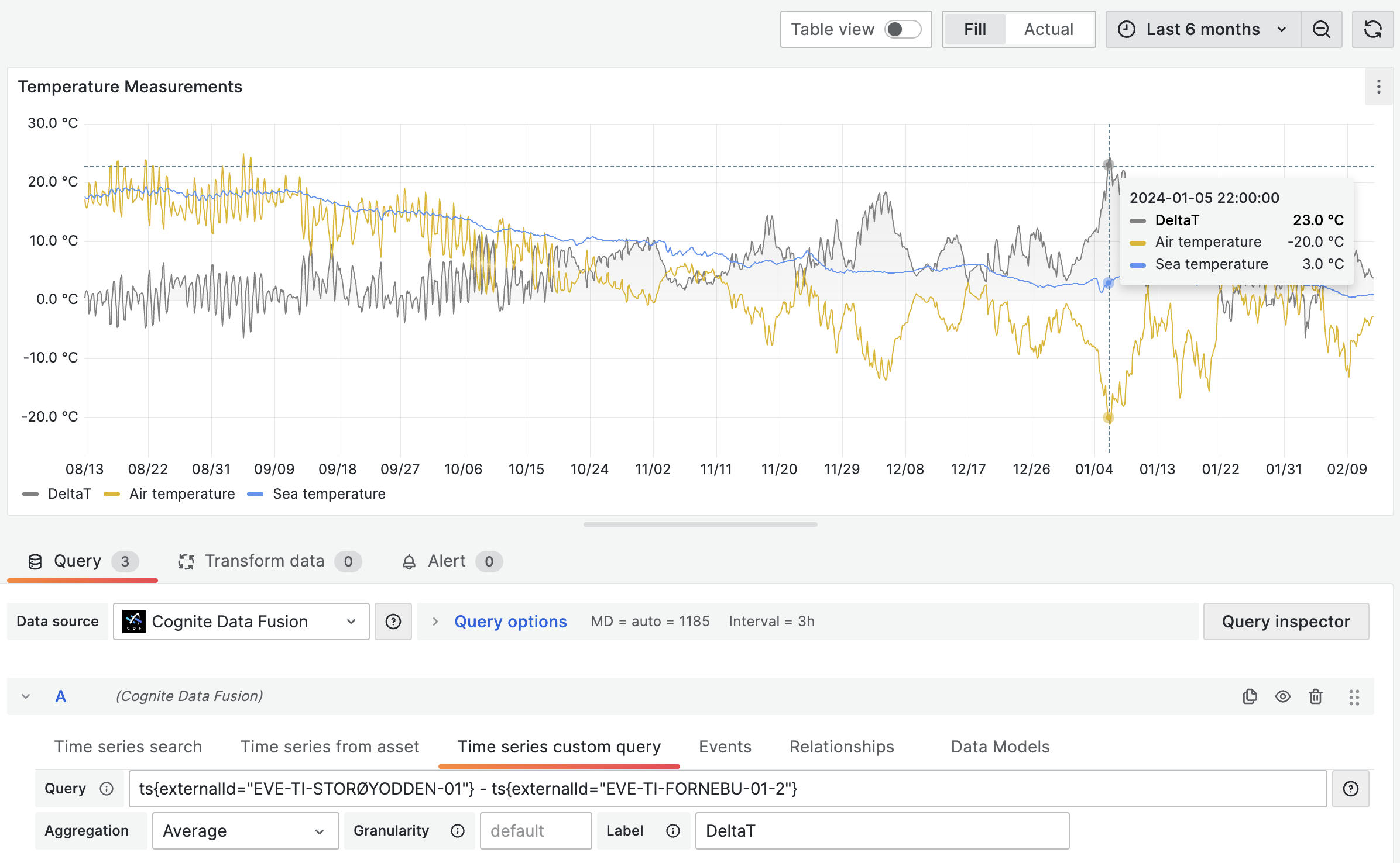
### Arithmetic operations
You can apply arithmetic operations to combine time series. For example:
```text theme={"languages":{"custom":["/_languages/kuiper.json","../_languages/kuiper.json"]}}
ts{id=123} + ts{externalId="test"}
```
The result of the above query is a single plot where data points are summed values of each time series.
In this example, the query `ts{name~="test1.*"}` can return more than one time series, but let's assume that it returns three time series with IDs `111`, `222`, and `333`:
```text theme={"languages":{"custom":["/_languages/kuiper.json","../_languages/kuiper.json"]}}
ts{name~="test1.*"} + ts{id=123}
```
The result of the query is three plots, a combination of summed time series values returned by the first and second expressions in the query. The resulting plots represent these queries:
* `ts{id=111} + ts{id=123}`
* `ts{id=222} + ts{id=123}`
* `ts{id=333} + ts{id=123}`
You can see an example of this behavior (each `ts{}` expression returns two time series) in the image below (notice the labels below the chart).
For **synthetic time series**, you can specify several property types:
* `bool`: `ts{isString=true}` or `ts{isStep=false}`
* `string` or `number`: `ts{id=123}` or `ts{externalId='external_123'}`
* `array`: `ts{assetIds=[123, 456]}`
* `object`: `ts{metadata={key1="value1", key2="value2"}}`
To create complex synthetic time series, you can combine the types in a single query:
```text theme={"languages":{"custom":["/_languages/kuiper.json","../_languages/kuiper.json"]}}
ts{name="test", assetSubtreeIds=[{id=123}, {externalId="external_123"}]}
```
### Filtering
Queries also support filtering based on time series properties which apply as logical `AND`. For instance, the query below finds time series:
* that belong to an asset with an `id` that equals `123`
* where `name` starts with `"Begin"`
* where `name` doesn't end with `"end"`
* where `name` doesn't equal `"Begin query"`
```text theme={"languages":{"custom":["/_languages/kuiper.json","../_languages/kuiper.json"]}}
ts{assetIds=[123], name=~"Begin.*", name!~".*end", name!="Begin query"}
```
The query syntax contains different types of equality operators:
* `=` - strict equality. Specifies parameters for the time series request to CDF. Use with filtering attributes.
* `!=` - strict inequality. Filters fetched time series by properties that aren't equal to the string. Supports string, numeric, and boolean values.
* `=~` – regex equality. Filters the fetched time series by properties that match the regular expression. Supports string values.
* `!~` - regex inequality. Filters the fetched time series by properties that don't match the regular expression. Supports string values.
You can also filter on metadata:
```text theme={"languages":{"custom":["/_languages/kuiper.json","../_languages/kuiper.json"]}}
ts{externalIdPrefix="test", metadata={key1="value1", key2=~"value2.*"}}
```
The query above requests for time series where:
* `externalIdPrefix` equals `"test"`
* `metadata.key1` equals `"value1"`
* `metadata.key2` starts with `"value2"`
### Query limitations
When performing custom queries, it's important to understand the underlying limitations for fetching time series:
* **Client-side Filtering**: The connector applies regex queries (`=~` for matches and `!~` for exclusions) and inexact inequality filters (`!=`) on the *client-side*. This process occurs after the initial retrieval of up to 1000 time series items from Cognite Data Fusion (CDF). Due to this approach, there's a possibility that not all relevant time series will be included in the fetched subset if the total number exceeds 1000.
* **Server-side Filtering**: To mitigate this limitation, it's recommended to use *server-side* filtering whenever possible. This can be achieved by applying strict equality filters (`=`) on specific [time series filter properties](https://api-docs.cognite.com/20230101/tag/Time-series/operation/listTimeSeries/). By doing so, you effectively narrow down the set of time series retrieved from CDF, ensuring that the subsequent client-side filters are applied to a more targeted dataset. This is particularly useful for ensuring that all relevant time series, especially those of interest, are included within the initial dataset fetched from CDF.
Combine *server-side* filtering with specific attributes or metadata to refine your query's scope before applying *regex* or other *client-side* filters. This approach significantly increases the chances of selecting all time series of interest in your Grafana dashboard.
### Aggregation, granularity, and alignment
You can specify aggregation and granularity for each time series using the dropdowns in the user interface.
If, for example, the aggregation is set to `average` and the granularity equals `1h`, **all** queries request datapoints with the selected aggregation and granularity. By default, aggregation with synthetic time series is aligned to Thursday 00:00:00 UTC, 1 January 1970.
With the synthetic time series query syntax, you can define aggregation, granularity, and alignment for **each time series separately**:
```text theme={"languages":{"custom":["/_languages/kuiper.json","../_languages/kuiper.json"]}}
ts{externalId='houston.ro.REMOTE_AI[34]', alignment=1599609600000, aggregate='average', granularity='24h'}
```
The query above overrides the aggregation and granularity values set in the user interface. See the API documentation for a list of [supported aggregates](/api-reference/concepts/20230101/synthetic-time-series#aggregation).
### Arithmetic operations
You can apply arithmetic operations to combine time series. For example:
```text theme={"languages":{"custom":["/_languages/kuiper.json","../_languages/kuiper.json"]}}
ts{id=123} + ts{externalId="test"}
```
The result of the above query is a single plot where data points are summed values of each time series.
In this example, the query `ts{name~="test1.*"}` can return more than one time series, but let's assume that it returns three time series with IDs `111`, `222`, and `333`:
```text theme={"languages":{"custom":["/_languages/kuiper.json","../_languages/kuiper.json"]}}
ts{name~="test1.*"} + ts{id=123}
```
The result of the query is three plots, a combination of summed time series values returned by the first and second expressions in the query. The resulting plots represent these queries:
* `ts{id=111} + ts{id=123}`
* `ts{id=222} + ts{id=123}`
* `ts{id=333} + ts{id=123}`
You can see an example of this behavior (each `ts{}` expression returns two time series) in the image below (notice the labels below the chart).
 ### Functions
We support a wide range of functions that you can apply to synthetic time series:
* **Trigonometric:** `sin(ts{})`, `cos(ts{})`, `pi()`.
* **Variable-length functions:** `max(ts{}, ...)`, `min(ts{}, ...)`, `avg(ts{}, ...)`.
* **Algebraic:** `ln(ts{})`, `pow(ts{}, exponent)`, `sqrt(ts{})`, `exp(ts{})`, `abs(ts{})`.
* **Error handling**: `on_error(ts{}, default_value)`. See [Error handling for calculations](#error-handling-for-calculations).
* **String time series:** `map(expression, [list of strings to map from], [list of values to map to], default_value)`. See [String time series](#string-time-series).
### Error handling for calculations
The `on_error(ts{...})` function allows chart rendering even if some exception appears. It handles errors like:
* `BAD_DOMAIN` - If bad input ranges are provided. For example, division by zero, or the square root of a negative number.
* `OVERFLOW` - If the result is more than 10^100 in absolute value.
If any of these are encountered, instead of returning a value for the timestamp, CDF returns an error field with an error message. To avoid these, you can wrap the (sub)expression in the `on_error()` function:
```text theme={"languages":{"custom":["/_languages/kuiper.json","../_languages/kuiper.json"]}}
on_error(1/ts{externalId='canBeZero'}, 0)
```
### String time series
The `map()` function can handle time series with string values to convert strings to doubles. If, for example, a time series for a valve can have the values `"OPEN"` or `"CLOSED"`, you can convert it to a number with:
```text theme={"languages":{"custom":["/_languages/kuiper.json","../_languages/kuiper.json"]}}
map(TS{externalId='stringstate'}, ['OPEN', 'CLOSED'], [1, 0], -1)
```
`"OPEN"` is mapped to 1, `"CLOSED"` to 0, and everything else to -1.
Aggregates on string time series are currently not supported. All string time series are considered to be stepped time series.
### Unit conversion
If a time series has a defined `unitExternalId`, you can convert its values to a different unit within the same quantity when querying data using custom queries.
Example:
```text theme={"languages":{"custom":["/_languages/kuiper.json","../_languages/kuiper.json"]}}
{ts{externalId='temperature_f_houston', targetUnit='temperature:deg_c'} + ts{id='123', targetUnitSystem='SI'}}
```
You can choose either `targetUnit` or `targetUnitSystem` for each time series or aggregate. The target unit you choose must be compatible with the original unit.
When querying data points using synthetic time series, the units for the values will not be kept. This means it's possible to add values from a **temperature** time series to a **distance** time series, even though it's not physically accurate.
If you try to access the `unit` or `unitExternalId` properties of each time series on the **label** field, Grafana will return the original unit of the time series, not the unit of the data points.
### Functions
We support a wide range of functions that you can apply to synthetic time series:
* **Trigonometric:** `sin(ts{})`, `cos(ts{})`, `pi()`.
* **Variable-length functions:** `max(ts{}, ...)`, `min(ts{}, ...)`, `avg(ts{}, ...)`.
* **Algebraic:** `ln(ts{})`, `pow(ts{}, exponent)`, `sqrt(ts{})`, `exp(ts{})`, `abs(ts{})`.
* **Error handling**: `on_error(ts{}, default_value)`. See [Error handling for calculations](#error-handling-for-calculations).
* **String time series:** `map(expression, [list of strings to map from], [list of values to map to], default_value)`. See [String time series](#string-time-series).
### Error handling for calculations
The `on_error(ts{...})` function allows chart rendering even if some exception appears. It handles errors like:
* `BAD_DOMAIN` - If bad input ranges are provided. For example, division by zero, or the square root of a negative number.
* `OVERFLOW` - If the result is more than 10^100 in absolute value.
If any of these are encountered, instead of returning a value for the timestamp, CDF returns an error field with an error message. To avoid these, you can wrap the (sub)expression in the `on_error()` function:
```text theme={"languages":{"custom":["/_languages/kuiper.json","../_languages/kuiper.json"]}}
on_error(1/ts{externalId='canBeZero'}, 0)
```
### String time series
The `map()` function can handle time series with string values to convert strings to doubles. If, for example, a time series for a valve can have the values `"OPEN"` or `"CLOSED"`, you can convert it to a number with:
```text theme={"languages":{"custom":["/_languages/kuiper.json","../_languages/kuiper.json"]}}
map(TS{externalId='stringstate'}, ['OPEN', 'CLOSED'], [1, 0], -1)
```
`"OPEN"` is mapped to 1, `"CLOSED"` to 0, and everything else to -1.
Aggregates on string time series are currently not supported. All string time series are considered to be stepped time series.
### Unit conversion
If a time series has a defined `unitExternalId`, you can convert its values to a different unit within the same quantity when querying data using custom queries.
Example:
```text theme={"languages":{"custom":["/_languages/kuiper.json","../_languages/kuiper.json"]}}
{ts{externalId='temperature_f_houston', targetUnit='temperature:deg_c'} + ts{id='123', targetUnitSystem='SI'}}
```
You can choose either `targetUnit` or `targetUnitSystem` for each time series or aggregate. The target unit you choose must be compatible with the original unit.
When querying data points using synthetic time series, the units for the values will not be kept. This means it's possible to add values from a **temperature** time series to a **distance** time series, even though it's not physically accurate.
If you try to access the `unit` or `unitExternalId` properties of each time series on the **label** field, Grafana will return the original unit of the time series, not the unit of the data points.